在Barsky的程序中,有关Crank-Nicolson algorithm的算法,所以那来看了一下。以下是
1.摘自:http://sepwww.stanford.edu/sep/prof/bei/fdm/paper_html/node15.html
The Crank-Nicolson method
The Crank-Nicolson method solves both the accuracy and the stability problem. Recall the difference representation of the heat-flow equation (27).
| (29) |
Now, instead of expressing the right-hand side entirely at time t, it will be averaged at t and t+1, giving
| |
(30) |
This is called the Crank-Nicolson method. Defining a new parameter ![]() ,the difference star is
,the difference star is
 |
(31) |
When placing this star over the data table, note that, typically, three elements at a time cover unknowns. To say the same thing with equations, move all the t+1 terms in (30)
to the left and the t terms to the right, obtaining
| |
(32) |
Now think of the left side of equation (32) as containing all the unknown quantities and the right side as containing all known quantities. Everything
on the right can be combined into a single known quantity, say, dtx. Now we can rewrite equation (32) as a set of simultaneous
equations. For definiteness, take the x-axis to be limited to five points. Then these equations are:
![\begin{displaymath}\left[\matrix {\matrix { e_{\rm left} \cr - \alpha_{}^{}\c... ...rix {d_t^1 \cr d_t^2 \cr d_t^3 \cr d_t^4 \cr d_t^5 }}\right]\end{displaymath}](http://sepwww.stanford.edu/sep/prof/bei/fdm/paper_html/img88.gif) |
(33) |
Equation (32) does not give us each qt+1x explicitly, but equation (33)
gives them implicitly by the solution of simultaneous equations.
The values ![]() and
and ![]() are
are
adjustable and have to do with the side boundary conditions. The important thing to notice is that the matrix is tridiagonal, that is, except for three central diagonals all the elements of the matrix in (33)
are zero. The solution to such a set of simultaneous equations may be economically obtained. It turns out that the cost is only about twice that of the explicit method given by (27).
In fact, this implicit method turns out to be cheaper, since the increased accuracy of (32) over (27)
allows the use of a much larger numerical choice of ![]() .A program that demonstrates the stability of the method, even
.A program that demonstrates the stability of the method, even
for large ![]() , is given next.
, is given next.
A tridiagonal simultaneous equation solving subroutine rtris() explained in the next section. The results are stable, as you can see.
2.摘自:http://en.wikipedia.org/wiki/Crank%E2%80%93Nicolson_method
Crank–Nicolson method
In numerical analysis, the Crank–Nicolson
method is a finite difference method used for numerically solving the heat
equation and similar partial differential equations.[1] It
is a second-order method in time, it is implicit in
time and can be written as an implicit Runge–Kutta method, and it isnumerically
stable. The method was developed by John Crank and Phyllis
Nicolson in the mid 20th century.[2]
For diffusion equations (and many other equations), it can be shown the Crank–Nicolson method is unconditionally stable.[3] However,
the approximate solutions can still contain (decaying) spurious oscillations if the ratio of time step Δt times the thermal
diffusivity to the square of space step, Δx2, is large (typically larger than 1/2[citation
needed]). For this reason, whenever large time steps or high spatial resolution is necessary, the less accurate backward
Euler method is often used, which is both stable and immune to oscillations.
Contents[hide] |
[edit]The
method

The Crank–Nicolson method is based on central
difference in space, and the trapezoidal rule in time, giving second-order
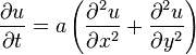
convergence in time. For example, in one dimension, if the partial differential equation is
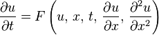
then, letting 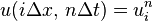 ,
,
the equation for Crank–Nicolson method is a combination of the forward Euler method at  and
and
the backward Euler method at n + 1 (note, however, that the method itself is not simply the average
of those two methods, as the equation has an implicit dependence on the solution):


![\frac{u_{i}^{n + 1} - u_{i}^{n}}{\Delta t} = \frac{1}{2}\left[F_{i}^{n + 1}\left(u,\, x,\, t,\, \frac{\partial u}{\partial x},\, \frac{\partial^2 u}{\partial x^2}\right) + F_{i}^{n}\left(u,\, x,\, t,\, \frac{\partial u}{\partial x},\, \frac{\partial^2 u}{\partial x^2}\right)\right] \qquad \mbox{(Crank-Nicolson)}.](http://upload.wikimedia.org/math/9/e/5/9e5ba7f3f8a51dee5a74904f54ad2fdc.png)
The function F must be discretized spatially with a central
difference.
Note that this is an implicit method: to get the "next" value of u in time, a system of algebraic equations must be solved. If the partial differential equation is nonlinear,
the discretization will also be nonlinear so that advancing in time will involve the solution of a system of nonlinear algebraic equations, though linearizations are possible. In many problems, especially linear diffusion, the algebraic problem is tridiagonal and
may be efficiently solved with thetridiagonal matrix algorithm, which gives a fast  direct
solution as opposed to the usual  for a full matrix.
[edit]Example:
1D diffusion
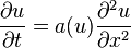
The Crank–Nicolson method is often applied to diffusion
problems. As an example, for linear diffusion,

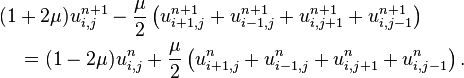
whose Crank–Nicolson discretization is then:

or, letting  :
:

which is a tridiagonal problem, so that  may
may
be efficiently solved by using the tridiagonal matrix algorithm in favor of a much more costly matrix
inversion.
A quasilinear equation, such as (this is a minimalistic example and not general)
would lead to a nonlinear system of algebraic equations which could not be easily solved as above; however, it is possible in some cases to linearize the problem by using the old value for  ,
,
that is  instead of
  .
.
Other times, it may be possible to estimate using an explicit method
and maintain stability.
[edit]Example:
1D diffusion with advection for steady flow, with multiple channel connections
This is a solution usually employed for many purposes when there's a contamination problem in streams or rivers under steady flow conditions but information is given in one dimension only.
Often the problem can be simplified into a 1-dimensional problem and still yield useful information.
Here we model the concentration of a solute contaminant in water. This problem is composed of three parts: the known diffusion equation ( chosen
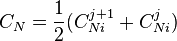
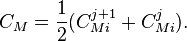
as constant), an advective component (which means the system is evolving in space due to a velocity field), which we choose to be a constant Ux, and a lateral interaction between longitudinal channels (k).
-

(
where C is the concentration of the contaminant and subscripts N and M correspond to previous and next channel.
The Crank–Nicolson method (where i represents position and j time) transforms each component of the PDE into the following:
-
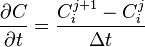
(
-

(
-

(
-

(
-
(
-
(
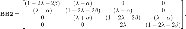
Now we create the following constants to simplify the algebra:


and substitute (2),
(3), (4),
(5), (6),
(7), α, β and λ into (1).
We then put the new time terms on the left (j + 1) and the present time terms on the right (j) to get:

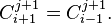
To model the first channel, we realize that it can only be in contact with the following channel (M), so the expression is simplified to:

In the same way, to model the last channel, we realize that it can only be in contact with the previous channel (N), so the expression is simplified to:

To solve this linear system of equations we must now see that boundary conditions must be given first to the beginning of the channels:
 : initial condition
for the channel at present time step : initial condition for the channel at next time step
 : initial condition for the previous channel to the one analyzed at present time
step : initial condition for the next channel to the one analyzed at present time
step.
For the last cell of the channels (z) the most convenient condition becomes an adiabatic one, so

This condition is satisfied if and only if (regardless of a null value)
Let us solve this problem (in a matrix form) for the case of 3 channels and 5 nodes (including the initial boundary condition). We express this as a linear system problem:
![\begin{bmatrix}AA\end{bmatrix}\begin{bmatrix}C^{j+1}\end{bmatrix}=[BB][C^{j}]+[d]](http://upload.wikimedia.org/math/0/c/3/0c33d6714679e2ac59da34af149d6dc2.png)
where
-

and
Now we must realize that AA and BB should be arrays made of four different subarrays (remember that only three channels are considered for this example but it covers the main
part discussed above).
-
 and
and
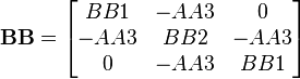
where the elements mentioned above correspond to the next arrays and an additional 4x4 full of zeros. Please note that the sizes of AA and BB are 12x12:
-

,
-

,
-

,
-

&
The d vector here is used to hold the boundary conditions. In this example it is a 12x1 vector:

To find the concentration at any time, one must iterate the following equation:
![\begin{bmatrix}C^{j+1}\end{bmatrix}=\begin{bmatrix}AA^{-1}\end{bmatrix}([BB][C^{j}]+[d]).](http://upload.wikimedia.org/math/6/b/9/6b98e2da9d71fa7b5f8e55c9e7068780.png)
[edit]Example:
2D diffusion
When extending into two dimensions on a uniform Cartesian
grid, the derivation is similar and the results may lead to a system of band-diagonal equations rather
than tridiagonal ones. The two-dimensional heat equation
can be solved with the Crank–Nicolson discretization of
![\begin{align}u_{i,j}^{n+1} &= u_{i,j}^n + \frac{1}{2} \frac{a \Delta t}{(\Delta x)^2} \big[(u_{i+1,j}^{n+1} + u_{i-1,j}^{n+1} + u_{i,j+1}^{n+1} + u_{i,j-1}^{n+1} - 4u_{i,j}^{n+1}) \\ & \qquad {} + (u_{i+1,j}^{n} + u_{i-1,j}^{n} + u_{i,j+1}^{n} + u_{i,j-1}^{n} - 4u_{i,j}^{n})\big]\end{align}](http://upload.wikimedia.org/math/6/2/d/62d1c1169a9b3e9ea7866097dcc0746b.png)
assuming that a square grid is used so that  .
.
This equation can be simplified somewhat by rearranging terms and using the CFL number

For the Crank–Nicolson numerical scheme, a low CFL
number is not required for stability, however it is required for numerical accuracy. We can now write the scheme as:
[edit]Application
in financial mathematics
Because a number of other phenomena can be modeled with
the heat equation (often called the diffusion equation in financial
mathematics), the Crank–Nicolson method has been applied to those areas as well.[4] Particularly,
the Black–Scholes option pricing model's differential
equation can be transformed into the heat equation, and thus numerical solutions for option
pricing can be obtained with the Crank–Nicolson method.
The importance of this for finance, is that option pricing problems, when extended beyond the standard assumptions (e.g. incorporating changing dividends), cannot be solved in closed form,
but can be solved using this method. Note however, that for non-smooth final conditions (which happen for most financial instruments), the Crank–Nicolson method is not satisfactory as numerical oscillations are not damped. For vanilla
options, this results in oscillation in thegamma value around the strike
price. Therefore, special damping initialization steps are necessary (e.g., fully implicit finite difference method).
[edit]See
also
[edit]References
- ^ Tuncer
Cebeci (2002). Convective Heat Transfer. Springer. ISBN 0-9668461-4-1. - ^ Crank,
J.; Nicolson, P. (1947). "A practical method for numerical evaluation of solutions of partial differential equations of the heat conduction type". Proc. Camb. Phil. Soc.43 (1): 50–67. doi:10.1007/BF02127704.. - ^ Thomas,
J. W. (1995). Numerical Partial Differential Equations: Finite Difference Methods. Texts in Applied Mathematics. 22. Berlin, New York: Springer-Verlag. ISBN 978-0-387-97999-1..
Example 3.3.2 shows that Crank–Nicolson is unconditionally stable when applied to .
. - ^ Wilmott,
P.; Howison, S.; Dewynne, J. (1995). The
Mathematics of Financial Derivatives: A Student Introduction. Cambridge Univ. Press. ISBN 0-521-49789-2.