学步园

INTRODUCTION
In recent years, estimation techniques that use time series cross-sectional (panel) data approaches have become widely used. The PANEL procedure in SAS/ETS software fits classes of linear models that arise when time series and cross-sectional data are combined.
It is capable of fitting the following models:

• one-way and two-way models
• random-effects and fixed-effects models
• autoregressive and moving average models
   o Parks method
   o dynamic panel method (GMM)
   o Da Silva method

This paper uses simulated data to compare these techniques and outline their advantages and disadvantages. The paper starts with a brief theoretical overview of panel data methods. Several examples are given to demonstrate these techniques and their implementation
in the PANEL procedure. The PANEL procedure is then compared with other SAS procedures.

PANEL MODELS
In this paper, the term panel refers to pooled data on time series cross-sectional bases. Typical examples of panel data include observations on households, countries, firms, trade, etc. For example, in the case of survey data on household income,
the panel is created by repeatedly surveying the same households in different time periods
(years). The model is typically written in the following form:

Even though the dynamic nature of the model reflects the real relationship between the independent and dependent variables more accurately, the introduction of the lagged dependent variable can pose a variety of problems. Given the model structure, the dependent
variables y(it) and y(it-1) are functions of  μ(i) , and estimation using ordinary least squares (OLS) will result in biased, inefficient, and inconsistent estimates. As discussed by Baltagi (1995), other models specifically designed for panel data also suffer
from efficiency issues. This paper uses the PANEL procedure to demonstrate issues that might arise with a model that is dynamic in nature. ODS Graphics plots are used to
demonstrate results from various models.

DATA GENERATING PROCESS
The following AR(1) panel data generating process (DGP) was adopted from Bond, Bowsher, and Windmeijer (2001). One hundred cross sections, each containing six time periods, were generated. The DGP can be described as follows:

data two;
delta = 0.4;
array x[6];
do i=1 to 100;/*i从1到100*/
   e_i = 4*rannor(1234);/*N(O,4)*/
   mu_i = 36*rannor(32444);/*N(0,36)*/
   do t=1 to 6;/*t从1到6*/
      do k = 1 to 6;
         x[k] = 3+4*(rannor(58785));/*系数β=3*/
      end;
   if t = 1 then 
      y = mu_i/(1-delta) + x1 + 5*x2 +10*x3 + e_i;/*β=5*/
   else do;
      v_it = 4*rannor(34454);
      y = delta * y_t1 + mu_i + x1 + 5*x2 +10*x3 + v_it;
   end;
   output;
   y_t1 = y;
   end;
end;
run;

MODEL ESTIMATION
When introduced to a new method, users are likely to compare it with other estimation frameworks and techniques that are available. In this section, the generated data are used and several different models are estimated. We start with a simple OLS model that
ignores the time series cross-sectional nature of the data by using the REG procedure.

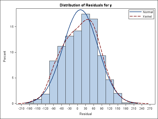
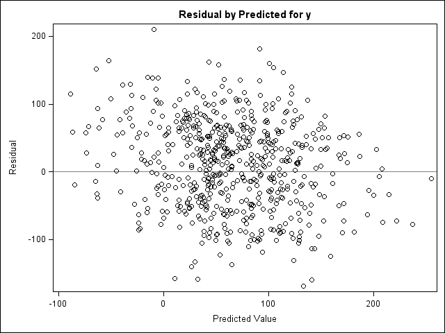
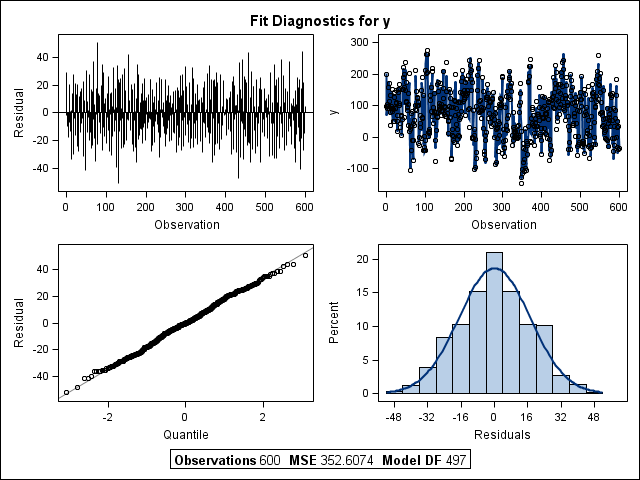
ods graphics on;
proc reg data = two plot(unpackpanel)=all;
model y = x1 x2 x3 /noint;
run;
ods graphics off;

The model is estimated for three different cross-sectional error specifications, and the new PLOT option is used to obtain fit diagnostics for residuals (Figure 1).

Using the following statements, one-way fixed- and random-effects models are estimated using the PANEL procedure for the same three cross-sectional error specifications:

ods graphics on;
proc panel data = two plot=all;
id i t;
model y =x1 x2 x3 /fixone ranone noint;
run;
ods graphics off;

The PLOT=ALL option is used to obtain two diagnostic panels to examine the fit of the model. The panels for the oneway random-effects model are presented in Figures 2 and 3. The first panel was created using all 100 cross sections; the second
panel depicts only the first 10 cross sections.

 Since the model specification in Equation (2) includes a lagged dependent variable,One-way to correct for the inefficiencies is by using GMM for panel models developed by Arellano and Bond (1991), as follows :

ods graphics on;
proc panel data=two plot(unpackpanel)=all;
id i t;
instrument depvar exogenous = (x4 x5 x6);
model y =  x1 x2 x3 /gmm twostep maxband=5 nolevels noint;
run;
ods graphics off;

It can be clearly seen from Equation (2) that the dependent variable y is not exogenous, since its values depend on its previous realizations. Arellano and Bond (1991) show that the dependent variable can still be used as one of the instruments
if properly lagged. This is accomplished by using the DEPVAR option in the INSTRUMENT statement.
The INSTRUMENT statement can include other variables that are not correlated with the error term. In this model, x4, x5, and x6 are considered to be purely exogenous and uncorrelated with the error. In other models, it is possible that future values of available
instruments are correlated with the error term but their past and current realizations are not. The fact that the past and present realizations are not correlated with the error enables us to use them as instruments with the PREDETERMINED option. The following
INSTRUMENT statement is used to describe a model with two exogenous and one predetermined variables:

instrument depvar exogenous = (x4 x5) predetermined = (x6);

The Arellano and Bond method is very useful in dealing with autoregressive data. It is important to realize, however, that using too many instruments can produce biased parameter estimates and cause computational difficulties since the weighting
matrix becomes very large. In Arellano and Bond’s original paper, only the past values of dependent variable are used as instruments. In theory, any variables that are not correlated with the error can be used. However, you have to make sure that the selected
instruments are strong and that the model is not misspecified. Inclusion of unnecessary instruments can be partially prevented with the MAXBAND option. Results of the GMM estimation with x4, x5, and x6 specified as exogenous variables are presented in Table
4.

 PANEL PROCEDURE AND SAS
The new PANEL procedure enhances the features that were implemented in the TSCSREG procedure. The new methods added include between estimators, pooled estimators, and dynamic panel estimators using GMM. The CLASS statement creates classification variables
that are used in the analysis. The FLATDATA statement allows the data to be in a compress form. The TEST statement includes new options for Wald, Lagrange multiplier, and likelihood ratio tests. Since the presence of heteroscedasticity can result in inefficient
and biased estimates of the variance covariance matrix in the OLS framework, several methods producing heteroscedasticity-consistent covariance matrices (HCCME) were added. The new RESTRICT statement specifies linear restrictions on the parameters. The PANEL
procedure now produces graphical displays by using ODS Graphics. The new plots include residual, predicted, and actual value plots, Q-Q plots, histograms, and profile plots. The OUTPUT statement enables the user to output data and estimates that can be used
in other analysis. It is typically difficult to create lagged variables in the panel setting. If lagged variables are created in a DATA step, several programming steps including loops are often needed. The PANEL procedure makes creating lagged values easy
by including the LAG statement. The LAG statement, depending on the lag order, can generate a large number of missing values. The PANEL procedure offers a solution to the loss of potentially useful observations by replacing the missing values with zeros, overall
mean, time mean, or cross section mean (LAG, ZLAG, XLAG, SLAG, and CLAG statements).

The following SAS statements are used to create lagged values:

proc panel data=new;
   lag y(1) / out=test;
   id i t;
run;

Even though the new PANEL procedure represents a collection of powerful analytical and visual tools, it is important to remember that other procedures available in SAS/ETS and SAS/STAT software can include models that are not implemented in the PANEL procedure.
The LOGISTIC procedure offers fixed-effects models with nonnormal errors in panel setting. The NLMIXED procedure offers an implementation of nonlinear fixed- and random-effects models. The GLIMMIX procedure offers the most complete alternative for both fixed-
and random-effects models in linear and nonlinear settings. Other procedures offer the same types of models. For example, it is possible to fit a two-way random-effects model by using the MIXED procedure as follows:

proc mixed data=two method=type3;
   class i t;
   model y = x1 x2 x3 /solution;
   random i t;
run;

The same model can be estimated using the PANEL procedure as follows:

proc panel data=two;
   model y = x1 x2 x3 / rantwo vcomp = fb;
   id i t;
run;

Fixed-effects models are typically easy to implement through the use of dummy variables in many SAS procedures. The random-effects models are more complex and require specialized procedures. Methods available in the PANEL procedure along with a list of procedure
handling time series cross-sectional data are depicted in Figure 8. New additions that are available only in the PANEL procedure are shown in green.

CONCLUSION
This paper demonstrated the use of the new PANEL procedure in SAS/ETS software. It used simulated data with known parameter values to show advantages and disadvantages of different methods. Graphical displays produced  using ODS Graphics were used to diagnose
the fit of different models and correct for data distortion.

It is no surprise that OLS performed relatively poorly, because it ignores the time series cross-sectional nature of data. Using a simulation it was shown that a proper method, including one-way fixed or random effects, can correct for the estimate bias.
If heteroscedasticity is present, the PANEL procedure offers several ways to correct for it. If the data are dynamic in nature, the PANEL procedure offers the Arellano and Bond GMM method to regain efficiency. It is important to remember that additional tools
not available in the PANEL procedure can be found in other SAS/ETS SAS/STAT procedures. For example, the LOGISTIC procedure offers fixed-effects models with nonnormal errors. Nonlinear models can be estimated using the NLMIXED procedure.