Data Step Hash Objects as Programming Tools
Paul M. Dorfman, Independent Consultant, Jacksonville, FL
Koen Vyverman, SAS Netherlands
ABSTRACT
In SAS® Version 9.1, the hash table - the very first object introduced via the Data Step Component Interface in Version 9.0 - has become robust and syntactically stable. The philosophy and application style of the hash objects differs quite radically from
any other structure ever used in the Data step previously. The most notable departure from the tradition is their run-time nature. The hash objects are instantiated and/or deleted and acquire memory, if necessary, at the run-time. It is intuitively clear that
such traits should make for very interesting and flexible programming having not seen in the Data step code of yore.
Although some propaedeutics will be provided in the paper, the talk is intended for SAS programmers already somewhat familiar with the basic ideas and syntax behind the hash objects. Instead of teaching hash basics - which by now has been rehashed enough!
– live code examples will be used to demonstrate a number of programming techniques, which would be utterly unthinkable before the advent of the canned hash objects in SAS. Imagine using “data _null_” to write a SAS data set, whose name depends on a variable.
Or fancy sorting a huge temporary array rapidly and efficiently without the need for sophisticated hand-coding.
In other words, you are in for a few intriguing SAS tunes from the hash land.
INTRODUCTION
In the title of the paper, the term “hashing” was used collectively to denote the whole group of memory-resident searching methods not primarily based on comparison between keys, but on direct addressing. Although hashing per se is, strictly speaking, merely
one of direct-addressing techniques, using the word as a collective term has become quite common. Hopefully, it will be clear from the context in which sense the term is used. Mostly, it will be used in its strict meaning.
From the algorithmic standpoint, hashing is by no means a novel scheme, nor it is new in the SAS land. In fact, a number of direct-addressing searching techniques have been successfully implemented using the Data step language and shown to be practically
useful! This set of hand-coded direct-addressing routines, together with a rather painful delving into their guts, was presented at SUGI 26 and 27 [1, 2].
Hand-coded methods have a number of drawbacks – inevitable for almost any more or less complex, performance-oriented routine coded in a very high-level language, such as the SAS Data step. But it has a number of advantages as well, primarily that the code
is available, and so it can be tweaked to anyone’s liking, changed to accommodate different specifications, retuned, etc.
SAS Version 9 has introduced many new features into the Data step language. Most of them expand existing functionality and/or improve performance, and thus are rather incremental. However, one novel concept stands out as a breakthrough: The Data step Component
Interface. The two first objects available through this interface to a Data step programmer are associative array (or hash object) and the associated hash iterator object. These objects can be used as a memory-resident dynamic Data step dictionaries, which
can be created and deleted at the run time and perform the standard operations of finding, adding, and removing data practically in O(1) time. Being adroitly implemented in the underlying SAS software, these modules are quite fast, and the fact that memory
they need to store data is allocated dynamically, at the run time, makes the hash objects a real breakthrough.
HASH OBJECT AB OVO BY EXAMPLE: FILE MATCHING
Perhaps the best way to get a fast taste of this mighty addition to the Data step family is to see how easily it can help solve the “matching problem”. Suppose we have a SAS file LARGE with $9 character key KEY, and a file SMALL with a similar key and some
additional info stored in a numeric variable S_SAT. We need to use the SMALL file as a fast lookup table to pull S_SAT into LARGE for each KEY having a match in SMALL. This step shows one way how the hash (associative array) object can help solve the problem:
Example 1: File Matching (Lookup file loaded in a loop)
data match ( drop = rc ) ;
length key $9 s_sat 8 ;
declare AssociativeArray hh () ;
rc = hh.DefineKey ( 'key' ) ;
rc = hh.DefineData ( 's_sat' ) ;
rc = hh.DefineDone () ;
do until ( eof1 ) ;
set small end = eof1 ;
rc = hh.add () ;
end ;
do until ( eof2 ) ;
set large end = eof2 ;
rc = hh.find () ;
if rc = 0 then output ;
end ;
stop ;
run ;
After all the trials and tribulations of coding hashing algorithms by hand, this simplicity looks rather stupefying. But how does this code go about its business?
• LENGTH statement gives SAS the attributes of the key and data elements before the methods defining them could be called.
• DECLARE AssociativeArray statement declares and instantiates the associative array (hash table) HH.
• DefineKey method describes the variable(s) to serve as a key into the table.
• DefineData method is called if there is a non-key satellite information, in this case, S_SAT, to be loaded in the table.
• DefineDone method is called to complete the initialization of the hash object.
• ADD method grabs a KEY and S_SAT from SMALL and loads both in the table. Note that for any duplicate KEY coming from SMALL, ADD() will return a non-zero code and discard the key, so only the first instance the satellite
corresponding to a non-unique key will be used.
• FIND method searches the hash table HH for each KEY coming from LARGE. If it is found, the return code is set to zero, and host S_SAT field is updated with its value extracted from the hash table.
If you think it is prorsus admirabile, then the following step does the same with even less coding:
Example 2: File Matching (Lookup file is loaded via the DATASET: parameter)
data match ; set small point = _n_ ; * get key/data attributes for parameter type matching ; * set small (obs = 1) ; * this will work, too :-)! ; * if 0 then set small ; * and so will this :-)! ; * set small (obs = 0) ; * but for some reason, this will not; dcl hash hh (dataset: 'work.small', hashexp: 10) ; hh.DefineKey ( 'key' ) ; hh.DefineData ( 's_sat' ) ; hh.DefineDone () ; do until ( eof2 ) ; set large end = eof2 ; if hh.find () = 0 then output ; end ; stop ; run ;
Here are notable differences:
• Instead of the LENGTH statement, we can give the Define methods key and data attributes by reading a record from SMALL. Somewhat surprisingly, is not sufficient just to read a descriptor; there must be a record read at run-time.
• DCL can be used as a shorthand for
DECLARE.
• Keyword HASH can be used as an alias instead ofASSOCIATIVEARRAY. To the delight of those of us typo-impaired, it means: When people speak, SAS listens!
• Instead of loading keys and satellites from SMALL one datum at a time, we can instruct the hash table constructor to load the table directly from the SAS data file SMALL by specifying the file in the hash declaration.
• The object parameter HASHEXP tells the table constructor to allocate 2**10=1024 hash buckets.
• Assigning return codes to a variable when the methods are called is not mandatory. Omitting the assignments shortens notation.
NOTE 1: Parameter Type Matching
The LENGTH statement in the first version of the step or the attribute-extracting SET in the second one provide for what is called parameter type matching. When a method, such as FIND, is called, it presumes that a variable into which it can return a value
matches the type and length FIND expects it to be.
It falls squarely upon the shoulders of the programmer to make sure parameter types do match. The LENGTH or SET statements above achieve the goal by giving the table constructor the names of existing Data step variables for the key (KEY, length $9) and satellite
data (S_SAT, length 8).
Doing so simultaneously creates Data step host variable S_SAT, into which the FIND method (and others, as we will see later in the iterator section) automatically copies a value retrieved from the table in the case of a successful search.
NOTE 2: Handling Duplicate Keys
When a hash table is loaded from a data set, SAS acts as if the ADD method were used, that is, all duplicate key entries but the very first are ignored. Now, what if in the file SMALL, duplicated keys corresponded to different satellite values, and we needed
to pull the last instance of the satellite?
With hand-coded hash schemes, duplicate-key entries can be controlled programmatically by twisting the guts of the hash code. To achieve the desired effect using the hash object, we should call the REPLACE method instead of the ADD method. But to do so,
we have to revert back to the loading of the table in a loop one key entry at a time:
do until ( eof1 ) ;
set small end = eof1 ;
hh.replace () ;
end ;
Note that at this point, the hash object does not provide a mechanism of storing and/or handling duplicate keys with different satellites in the same hash table. This difficulty can be principally circumvented, if need be, by discriminating the primary key
by creating a secondary key from the satellite, thus making the entire composite key unique. Such an approach is aided by the ease with which hash tables can store and manipulate composite keys.
NOTE 3: Composite Keys and Multiple Satellites
In pre-V9 days, handling composite keys in a hand-coded hash table could be a breeze or a pain, depending on the type, range, and length of the component keys [1]. But in any case, the programmer needed to know the data beforehand and often demonstrate a
good deal of ingenuity.
The hash object makes it all easy. The only thing we need to do in order to create a composite key is define the types and lengths of the key components and instruct the object constructor to use them in the specified subordinate sequence. For example, if
we needed to create a hash table HH keyed by variables defined as
length k1 8 k2 $3 k3 8 ;
and in addition, had multiple satellites to store, such as
length a $2 b 8 c $4 ;
we could simply code:
dcl hash hh () ;
hh.DefineKey ('k1', 'k2', 'k3') ;
hh.DefineData ('a', 'b', 'c') ;
hh.DefineDone () ;
and the internal hashing scheme will take due care about whatever is necessary to come up with a hash bucket number where the entire composite key should fall together with its satellites.
Multiple keys and satellite data can be loaded into a hash table one element at a time by using the ADD or REPLACE methods. For example, for the table defined above, we can value the keys and satellites first and then call the ADD or REPLACE method:
k1 = 1 ; k2 = 'abc' ; k3 = 3 ;
a = 'a1' ; b = 2 ; c = 'wxyz' ;
rc = hh.replace () ;
k1 = 2 ; k2 = 'def' ; k3 = 4 ;
a = 'a2' ; b = 5 ; c = 'klmn' ;
rc = hh.replace () ;
Alternatively, these two table entries can be coded as
hh.replace (key: 1, key: 'abc', key: 3,
            data: 'a1', data: 2, data: 'wxyz') ;
hh.replace (key: 2, key: 'def', key: 4,
            data: 'a2', data: 5, data: 'klmn') ;
Note that more that one hash table entry cannot be loaded in the table at compile-time at once, as it can be done in the case of arrays. All entries are loaded one entry at a time at run-time.
Perhaps it is a good idea to avoid hard-coding data values in a Data step altogether, and instead always load them in a loop either from a file or, if need be, from arrays. Doing so reduces the propensity of the program to degenerate into an object Master
Ian Whitlock calls “wall paper”, and helps separate code from data.
NOTE 4: Hash Object Parameters as Expressions
The two steps above may have already given a hash-hungry reader enough to start munching overwhelming programming opportunities opened by the availability of the SAS-prepared hash food without the necessity to cook it. To add a little more spice to it, let
us rewrite the step yet another time:
Example 3: File Matching (Using expressions for parameters)
data match ;
   set small (obs = 1) ;
   retain dsn ‘small’ x 10 kn ‘key’ dn ‘s_sat’ ;
   dcl hash hh (dataset: dsn, hashexp: x) ;
   hh.DefineKey ( kn ) ;
   hh.DefineData ( dn ) ;
   hh.DefineDone ( ) ;
   do until ( eof2 ) ;
      set large end = eof2 ;
      if hh.find () = 0 then output ;
   end ;
   stop ;
run ;
As we see, the parameters passed to the constructor (such as DATASET and HASHEXP) and methods need not necessarily be hard-coded literals. They can be passed as valued Data step variables, or even as appropriate type expressions. For example, it is possible
to code (if need be):
retain args ‘small key s_sat’ n_keys 1e6;
dcl hash hh ( dataset: substr(args,1,5)
                   hashexp: log2(n_keys)
             ) ;
hh.DefineKey ( scan(s, 2) ) ;
hh.DefineData ( scan(s,-1) ) ;
hh.DefineDone ( ) ;
HITER: HASH ITERATOR OBJECT
During both hash table load and look-up, the sole question we need to answer is whether the particular search key is in the table or not. The FIND and CHECK hash methods give the answer without any need for us to know what other keys may or may not be stored
in the table. However, in a variety of situations we do need to know the keys and data currently resident in the table. How do we do that?
In hand-coded schemes, it is simple since we had full access to the guts of the table. However, hash object entries are not accessible as directly as array entries. To make them accessible, SAS provides the hash iterator object, hiter, which makes the hash
table entries available in the form of a serial list.
Let us consider a simple program that should make it all clear:
Example 4: Dumping the Contents of an Ordered Table Using the Hash Iterator
data sample ;
input k sat ;
cards ;
185 01
971 02
400 03
260 04
922 05
970 06
543 07
532 08
050 09
067 10
;
run ;
data _null_ ;
   if 0 then set sample ;
   dcl hash hh ( dataset: 'sample', hashexp: 8, ordered: 'a') ;
   dcl hiter hi ( 'hh' ) ;
   hh.DefineKey ( 'k' ) ;
   hh.DefineData ( 'sat' , 'k' ) ;
   hh.DefineDone () ;
   do rc = hi.first () by 0 while ( rc = 0 ) ;
      put k = z3. +1 sat = z2. ;
      rc = hi.next () ;
   end ;
   put 13 * '-' ;
   do rc = hi.last () by 0 while ( rc = 0 ) ;
      put k = z3. +1 sat = z2. ;
      rc = hi.prev () ;
   end ;
   stop ;
run ;
We see that now the hash table is instantiated with the ORDERED parameter set to ‘a’, which stands for ‘ascending’. When ‘a’ is specified, the table is automatically loaded in the ascending key order. It would be better to summarize the rest of the meaningful
values for the ORDERED parameter in a set of rules:
• ‘a’ , ‘ascending’ = ascending
• ‘y’ = ascending
• ‘d’ , ‘descending’ = descending
• ‘n’ = internal hash order (i.e. no order at all, and the original key order is NOT followed)
• any other character literal different from above = same as ‘n’
• parameter not coded at all = the same as ‘n’ by default
• character expression resolving to the same as the above literals = same effect as the literals
• numeric literal or expression = DSCI execution time object failure because of type mismatch
Note that the hash object symbol name must be passed to the iterator object as a character string, either hard-coded as above or as a character expression resolving to the symbol name of a declared hash object, in this case, “HH”. After the iterator HI has
been successfully instantiated, it can be used to fetch entries from the hash table in the key order defined by the rules given above.
To retrieve hash table entries in an ascending order, we must first point to the entry with the smallest key. This is done by the method FIRST:
rc = hi.first () ;
where HI is the name we have assigned to the iterator. A successful call to FIRST fetches the smallest key into the host variable K and the corresponding satellite - into the host variable SAT. Once this is done, each call to the NEXT method will fetch the
hash entry with the next key in ascending order. When no keys are left, the NEXT method returns RC > 0, and the loop terminates. Thus, the first loop will print in the log:
k=050 sat=09
k=067 sat=10
k=185 sat=01
k=260 sat=04
k=400 sat=03
k=532 sat=08
k=543 sat=07
k=922 sat=05
k=970 sat=06
k=971 sat=02
Inversely, the second loop retrieves table entries in descending order by starting off with the call to the LAST method fetching the entry with the largest key. Each subsequent call to the method PREV extracts an entry with the next smaller key until there
are no more keys to fetch, at which point PREV returns RC > 0, and the loop terminates. Therefore, the loop prints:
k=971 sat=02
k=970 sat=06
k=922 sat=05
k=543 sat=07
k=532 sat=08
k=400 sat=03
k=260 sat=04
k=185 sat=01
k=067 sat=10
k=050 sat=09
An alert reader might be curious why the key variable had to be also supplied to the DefineData method? After all, each time the DO-loop iterates the iterator points to a new key and fetches a new key entry. The problem is that the host key variable K is
updated only once, as a result of the HI.FIRST() or HI.LAST() method call. Calls to PREV and NEXT methods do not update the host key variable. However, a satellite hash variable does! So, if in the step above, it had not been passed to the DefineData method
as an additional argument, only the key values 050 and 971 would have been printed.
The concept behind such behavior is that only data entries in the table have the legitimate right to be “projected” onto its Data step host variables, whilst the keys do not. It means that if you need the ability to retrieve a key from a hash table, you need
to define it in the data portion of the table as well.
NOTE 5: Array Sorting via a Hash Iterator
The ability of a hash iterator to rapidly retrieve hash table entries in order is an extremely powerful feature, which will surely find a lot of use in Data step programming. The first iterator programming application that springs to mind immediately is
using its key ordering capabilities to sort another object. The easiest and most apparent prey is a SAS array. The idea of sorting an array using the hash iterator is very simple:
1. Declare an ordered hash table keyed by a variable of the data type and length same as those of the array.
2. Declare a hash iterator.
3. Assign array items one at a time to the key and insert the key in the table.
4. Use the iterator to retrieve the keys one by one from the table and repopulate the array, now in order.
A minor problem with this most brilliant plan, though, is that since the hash object table cannot hold duplicate keys, a certain provision ought to be made in the case the when the array contains duplicate elements. The simplest way to account for duplicate
array items is to enumerate the array as it is used to load the table and use the unique enumerating variable as an additional key into the table. In the case the duplicate elements need to be eliminated from the array, the enumerating variable can be merely
set to a constant, which below is chosen to be a zero:
Example 5: Using the Hash Iterator to Sort an Array
data _null_ ;
array a [-100000 : 100000] _temporary_ ;
** allocate sample array with random numbers, about 10 percent duplicate ;
do _q = lbound (a) to hbound (a) ;
a [_q] = ceil (ranuni (1) * 2000000) ;
end ;
** set sort parameters ;
seq = 'A' ; * A = ascending, D = descending ;
nodupkey = 0 ; * 0 = duplicates allowed, 1 = duplicates not allowed ;
dcl hash _hh (hashexp: 0, ordered: seq) ;
dcl hiter _hi ('_hh' ) ;
_hh.definekey ('_k', '_n' ) ; * _n - extra enumerating key ;
_hh.definedata ('_k' ) ; * _k automatically assumes array data type ;
_hh.definedone ( ) ;
** load composite (_k _n) key on the table ;
** if duplicates to be retained, set 0 <- _n ;
do _j = lbound (a) to hbound (a) ;
_n = _j * ^ nodupkey ;
_k = a [_j] ;
_hh.replace() ;
end ;
** use iterator HI to reload array from HH table, now in order ;
_n = lbound (a) - 1 ;
do _rc = _hi.first() by 0 while ( _rc = 0 ) ;
_n = _n + 1 ;
_rc = _hi.next() ;
end ;
_q = _n ;
** fill array tail with missing values if duplicates are delete ;
do _n = _q + 1 to hbound (a) ;
a [_n] = . ;
end ;
drop _: ; * drop auxiliary variables ;
** check if array is now sorted ;
sorted = 1 ;
do _n = lbound (a) + 1 to _q while ( sorted ) ;
if a [_n - 1] > a [_n] then sorted = 0 ;
end ;
put sorted = ;
run ;
Note that choosing HASHEXP:16 above would be more beneficial performance-wise. However, HASHEXP=0 was chosen to make an important point a propos:
Since it means 2**0=1, i.e. a single bucket, we have created a stand-alone AVL(Adelson-Volsky & Landis) binary tree in a Data step, let it grow dynamically as it was being populated with keys and satellites, and then traversed it to eject the data in a predetermined
key order. So, do not let anyone tell you that a binary search tree cannot be created, dynamically grown and shrunk, and deleted, as necessary at the Data step run time. It can, and with very a little programmatic effort, too!
Just to give an idea about this hash table performance in some absolute figures, this entire step runs in about 1.15 seconds on a desktop 933 MHz computer under XP Pro. The time is pretty deceiving, since 85 percent of it is spent inserting the data in the
tree. The process of sorting 200,001 entries itself takes only scant 0.078 seconds either direction. Increasing HASHEXP to 16 reduces the table insertion time by about 0.3 seconds, while the time of dumping the table in order remains the same.
One may ask why bother to program array sorting, even if the program is as simple and transparent as above, if in Version 9, CALL SORT() routine exists seemingly for the same purpose. In actuality, CALL SORT() is designed to sort variable lists, which may
or may not be organized into arrays. As such, it does not allow the provision of sorting a temporary array by a single array reference, unless all of its elements are explicitly listed. Of course, it is possible to assemble the references one by one using
a macro or another technique, but with 200001 elements to sort, it takes over 30 seconds just to compile the step. Besides, such method does not allow accounting for duplicates, and for those who care about such things, looks aesthetically maladroit.
DATA STEP COMPONENT INTERFACE
Now that we have a taste of the new Data step hash objects and some cool programming tricks they can be used to pull, let us consider it from a little bit more general viewpoint.
In Version 9, the hash table (associative array) introduces the first component object accessible via a rather novel thingy called DATA Step Component Interface (DSCI). A component object is an abstract data entity consisting of two distinct characteristics:
Attributes and methods. Attributes are data that the object can contain, and methods are operations the object can perform on its data
From the programming standpoint, an object is a black box with known properties, much like a SAS procedure. However, a SAS procedure, such as SORT or FORMAT, cannot be called from a Data step at run-time, while an object accessible through DSCI - can. A
Data step programmer who wants an object to perform some operation on its data, does not have to program it procedurally, but only to call an appropriate method.
The Hash Object
In our case, the object is a hash table. Generally speaking,as an abstract data entity,a hash table is an object providing for the insertion and retrieval of its keyed data entries in O(1),i.e. constant,time. Properly built direct-addressed tables satisfy
this definition in the strict sense. We will see that the hash object table satisfies it in the practical sense. The attributes of the hash table object are keyed entries comprising its key(s) and maybe also satellites.
Before any hash table object methods can be called (operations on the hash entries performed), the object must be declared. In other words, the hash table must be instantiated with the DECLARE (DCL) statement, as we have seen above.
The hash table methods are the functions it can perform, namely:
• DefineKey. Define a set of hash keys.
• DefineData. Define a set of hash table satelites.This method call can be omitted without harmful consequences if there is no need for non-key data in the table. Although a dummy call can be stil be issued,it is not required .
• DefineDone. Tell SAS the definitions are done. If the DATASET argument is passed to the table’s definition, load thetable from the data set.
• ADD. Insert the key and satellites if the key is not yet in the table (ignore duplicate keys). REPLACE. If the key is not in the table, insert the key and it satellites,otherwise overwrite the satellites in the table for this key with new ones.
• REMOVE. Delete the entire entry from the table, including the key and the data.
• FIND. Search for the key. If it is found,extract the satellite from the table and update the host Data step variable.
• CHECK. Search for the key. If it is found, just return RC=0, and do nothing more.Note that calling this method does not overwrite the host variables.
• OUTPUT. Dump the entire current contents of the table into a one or more SAS data set. Note that for the key(s) to dumped, they must be defined using the DefineData method. IF the table has been loaded in order, it will be dumped also in order. More information
about the method will be provided later on.
Data Step Object Dot Syntax
As we have seen, in order to call a method, we only have to specify its name preceded by the name of the object followed by a period, such as:
hh.DefineKey ()
h
h.Find () hh.Replace ()
hh.First ()
hh.Output ()
and so on. This manner of telling SAS Data step what to do is thus naturally called the Data Step Object Dot Syntax. Summarity,It provides a linguistic access to a component object's methods and attributes.
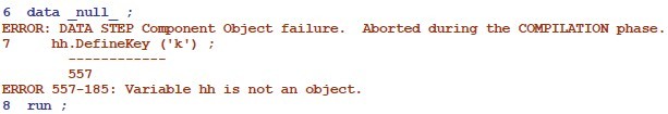
Note that the object dot syntax is one of very few things the Data step compiler knows about DSCI.The compile recognizes the syntax, and it reacts harshly if the dot syntax is resent, but the object to which it is apparently applied is absent. For example,
an attempt to compile this step,
data _null_ ;
hh.DefineKey ('k') ; run ;
results in the following log message from the compiler (not from the object):
So far, just a few component objects are accessible from a Data step through DSCI. However, as their number grows,we had better get used to the object dot syntax really soon, particularly those dinosaurs among us who have not exactly learnde this kind of
tongue in the kindergarten......