Refer from http://blog.sciencenet.cn/home.php?mod=space&uid=316653&do=blog&id=343366
Introduction
中文:自适应谐振理论
One of the nice features of human memory is its ability to learn many new things without necessarily forgetting things learned in the past. A frequently cited example is the ability to recognize your parents even if you have not seen them for some time and
have learned many new faces in the interim. It would be highly desirable if we could impart this same capability to an Artificial Neural Networks. Most neural networks will tend to forget old information if we attempt to add new information incrementally.
When developing an artificial neural network to perform a particular pattern-classification operation, we typically proceed by gathering a set of exemplars, or training patterns, then using these exemplars to train the system.
During the training, information is encoded in the system by the adjustment of weight values. Once the training is deemed to be adequate, the system is ready to be put into production, and no additional weight modification is permitted. This operational
scenario is acceptable provided the problem domain has well-defined boundaries and is stable. Under such conditions, it is usually possible to define an adequate set of training inputs for whatever problem is being solved. Unfortunately, in many realistic
situations, the environment is neither bounded nor stable. Consider a simple example. Suppose you intend to train abackpropagation
to recognize the silhouettes of a certain class of aircraft. The appropriate images can be collected and used to train the network, which is potentially a time-consuming task depending on the size of the network required. After the network has learned successfully
to recognize all of the aircraft, the training period is ended and no further modification of the weights is allowed. If, at some future time, another aircraft in the same class becomes operational, you may wish to add its silhouette to the store of knowledge
in your neural network. To do this, you would have to retrain the network with the new pattern plus all of the previous patterns. Training on only the new silhouette could result in the network learning that pattern quite well, but forgetting previously learned
patterns. Although retraining may not take as long as the initial training, it still could require a significant investment.
The Adaptative Resonance Theory: ART
In 1976, Grossberg (Grossberg, 1976) introduced a model for explaining biological phenomena. The model has three crucial properties:
- a normalisation of the total network activity. Biological systems are usually very adaptive to large changes in their environment. For example, the human eye can adapt itself to large variations in light intensities;
- contrast enhancement of input patterns. The awareness of subtle differences in input patterns can mean a lot in terms of survival. Distinguishing a hiding panther from a resting one makes all the difference in the world. The mechanism used here is contrast
enhancement; - short-term memory (STM,STM是指神经元的激活值.即末由s函数处理的输出值) storage of the contrast-enhanced pattern. Before the input pattern can be decoded, it must be stored in the short-term memory. The long-term memory (LTM,LTM是指权系数) implements an arousal(motivation) mechanism
(i.e., the classification), whereas the STM is used to cause gradual changes in the LTM.
The system consists of two layers, F1 and F2, which are connected to each other via the LTM
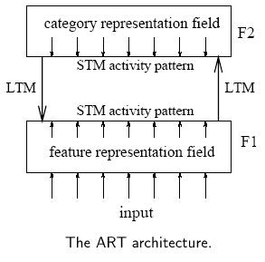
The input pattern is received at F1, whereas classification takes place in F2. As mentioned before, the input is not directly classified. First a characterisation takes place by means of extracting features, giving rise to activation in the feature representation
field. The expectations, residing in the LTM connections, translate the input pattern to a categorisation in the category representation field. The classification is compared to the expectation of the network, which resides in the LTM weights from F2 to F1.
If there is a match, the expectations are strengthened, otherwise the classification is rejected.
ART1: The simplified neural network model
The ART1 simplified model consists of two layers of binary neurons (with values 1 and 0), called F1 (the comparison layer) and F2 (the recognition layer)
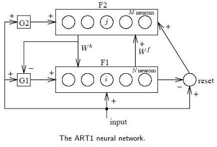
Each neuron in F1 is connected to all neurons in F2 via the continuous-valued forward long term memory (LTM) Wf , and vice versa via the binary-valued backward LTM Wb. The other modules are gain 1 and 2 (G1 and G2), and a reset module. Each neuron in the
comparison layer receives three inputs: a component of the input pattern, a component of the feedback pattern, and a gain G1. A neuron outputs a 1 if and only if at least two of these three inputs are high(+1)[3]: the 'two-thirds rule.' The neurons in the
recognition layer each compute the inner product of their incoming (continuous-valued) weights and the pattern sent over these connections. The winning neuron then inhibits all the other neurons via lateral inhibition. Gain 2 is the logical 'or' of all the
elements in the input pattern x. Gain 1 equals gain 2, except when the feedback pattern from F2 contains any 1; then it is forced to zero. Finally, the reset signal is sent to the active neuron in F2 if the input vector x and the output of F1 differ by more
than some vigilance(look with warning) level.
Operation
The network starts by clamping the input at F1. Because the output of F2 is zero, G1 and G2 are both on and the output of F1 matches its input.The pattern is sent to F2, and in F2 one neuron becomes active. This signal is then sent back over the backward
LTM, which reproduces a binary pattern at F1. Gain 1 is inhibited, and only the neurons in F1 which receive a 'one' from both x and F2 remain active. If there is a substantial mismatch between the two patterns, the reset signal will inhibit the neuron in F2
and the process is repeated.
- Initialisation:
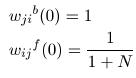 where N is the number of neurons in F1, M the number of neurons in F2, 0 ≤ i < N,
and 0 ≤ j <M. Also, choose the vigilance threshold ρ, 0 ≤ ρ ≤ 1; - Apply the new input pattern x:
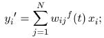
- compute the activation values y0 of the neurons in F2:
- select the winning neuron k (0 ≤ k <M):
- vigilance test: if
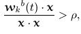 where . denotes inner product, go to step 7, else go to step 6. Note that
 essentially
is the inner product ,which will be large if
and near to each other;
 - neuron k is disabled from further activity. Go to step 3;
- Set for all l, 0 ≤ l < N:
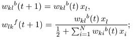
- re-enable all neurons in F2 and go to step 2.
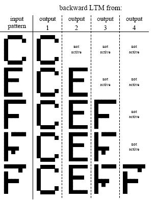
An example of the behaviour of the Carpenter Grossberg network for letter patterns. The binary input patterns on the left were applied sequentially. On the right the stored patterns (i.e., the weights of Wb for the first four output units) are shown.
ART1: The original model
In later work, Carpenter and Grossberg (Carpenter & Grossberg, 1987a, 1987b) present several neural network models to incorporate parts of the complete theory. We will only discuss the first model, ART1. The network incorporates a follow-the-leader clustering
algorithm (Hartigan, 1975). This algorithm tries to fit each new input pattern in an existing class. If no matching class can be found, i.e., the distance between the new pattern and all existing classes exceeds some threshold, a new class is created containing
the new pattern. The novelty in this approach is that the network is able to adapt to new incoming patterns, while the previous memory is not corrupted. In most neural networks, such as the backpropagation network, all patterns must be taught sequentially;
the teaching of a new pattern might corrupt the weights for all previously learned patterns. By changing the structure of the network rather than the weights, ART1 overcomes this problem.
More Reference:
[1] http://cns.bu.edu/Profiles/Grossberg/CarGro2003HBTNN2.pdf
[2] http://en.wikipedia.org/wiki/Adaptive_resonance_theory
[3] C++ neural networks and fuzzy logic.pdf-p99