LaTeX

This page outlines some more advanced uses of mathematics markup using LaTeX. In particular it makes heavy use of the AMS-LaTeX packages supplied by the American
Mathematical Society.

Contents   [hide]  1 Equation numbering 1.1 Subordinate equation numbering 2 Vertically aligning displayed mathematics 2.1 Above and below 2.2 align and align* 2.3 Braces spanning multiple lines 2.4 The cases environment 2.5 Other environments 3 Indented Equations 4 Page breaks in math environments 5 Boxed Equations 6 Custom operators 7 Advanced formatting 7.1 Limits 7.2 Subscripts and superscripts 7.3 Multiline subscripts 8 Text in aligned math display 9 Changing font size 10 Forcing \displaystyle for all math in a document 11 Notes

[edit]Equation
numbering

The equation environment automatically numbers your equation.

\begin{equation}   f(x)=(x+a)(x+b) \end{equation}

You can also use the \label and \ref (or \eqref from
the amsmath package) commands to label and reference equations, respectively. For equation number 1, \ref results
in and \eqref results
in :

\begin{equation} \label{eq:someequation} 5^2 - 5 = 20 \end{equation} this references the equation \ref{eq:someequation}.

\begin{equation} \label{eq:erl} a = bq + r \end{equation} where \eqref{eq:erl} is true if $a$ and $b$ are integers with $b \neq c$.

Further information is provided in the labels
and cross-referencing chapter.

To have the enumeration follow from your section or subsection heading, you must use the amsmath package or use AMS class documents.
Then enter

\numberwithin{equation}{section}

to the preamble to get enumeration at the section level or

\numberwithin{equation}{subsection}

to have the enumeration go to the subsection level.

\documentclass[12pt]{article} \usepackage{amsmath}  \numberwithin{equation}{subsection}  \begin{document}  \section{First Section}  \subsection{A subsection}  \begin{equation}   L' = {L}{\sqrt{1-\frac{v^2}{c^2}}}  \end{equation} \end{document}

If the style you follow requires putting dots after ordinals (as it is required at least in Polish typography) the \numberwithin{equation}{subsection} command
in preamble will result in the equation number in the above example to be rendered in this way: (1.1..1).

To remove the duplicate dot, add following command immediately after \numberwithin{equation}{subsection}:

\renewcommand{\theequation}{\thesection\arabic{equation}}

For numbering scheme using \numberwithin{equation}{subsection} use:

\renewcommand{\theequation}{\thesubsection\arabic{equation}}

in the preamble of the document.

Note: Though it may look like the \renewcommand works
by itself, it won't reset the equation number with each new section. It must be used together with manual equation number resetting after each new section beginning or with the much cleaner \numberwithin.

[edit]Subordinate
equation numbering

To number subordinate equations in a numbered equation environment, place the part of document containing them in a subequations environment:

\begin{subequations} Maxwell's equations: \begin{align}         B'&=-\nabla \times E,\\         E'&=\nabla \times B - 4\pi j, \end{align} \end{subequations}

Referencing of subordinate equations can be done in two methods. Adding a label after the \begin{subequations} command,
will reference to the main equation (1.1 the case presented). Adding a label after at the end of each line, before the \\ command,
will reference to the sub-equation (1.1a or 1.1b the case presented). It is possible to add both labels in case both types of references are needed.

[edit]Vertically
aligning displayed mathematics

An often encountered problem with displayed environments (displaymath and equation)
is the lack of any ability to span multiple lines. While it is possible to define lines individually, these will not be aligned.

[edit]Above
and below

The \overset and \underset commands^[1] typeset
symbols above and below expressions. Without AmsTex the same result of \overset can be obtained with \stackrel.
This can be particularly useful for creating new binary relations:

\[  A \overset{!}{=} B; A \stackrel{!}{=} B \]

or to show usage of L'Hôpital's
rule:

\[  \lim_{x\to 0}{\frac{e^x-1}{2x}}  \overset{\left[\frac{0}{0}\right]}{\underset{\mathrm{H}}{=}}  \lim_{x\to 0}{\frac{e^x}{2}}={\frac{1}{2}} \]

It's convenient to define a new operator that will set the equal sign with H and provided fraction:

\newcommand{\Heq}[1]{\overset{\left[#1\right]}{\underset{\mathrm{H}}{=}}}

to reduce above example to:

\[  \lim_{x\to 0}{\frac{e^x-1}{2x}}  \Heq{\frac{0}{0}}  \lim_{x\to 0}{\frac{e^x}{2}}={\frac{1}{2}} \]

If the purpose is to make comments on particular parts of an equation, the \overbrace and \underbrace commands
may be more useful, however they have a different syntax:

\[  z = \overbrace{    \underbrace{x}_\text{real} +    \underbrace{iy}_\text{imaginary}   }^\text{complex number} \]

Sometimes the comments are longer than the formula being commented on, which can cause spacing problems. These can be removed using the \mathclap command^[2]:

\[  y = a + f(\underbrace{b x}_{                     \ge 0 \text{ by assumption}})    = a + f(\underbrace{b x}_{           \mathclap{\ge 0 \text{ by assumption}}}) \]

Alternatively, to use brackets instead of braces use \underbracket and \overbracket commands^[2]:

\[  z = \overbracket[3pt]{      \underbracket{x}_{\text{real}} +      \underbracket[0.5pt][7pt]{iy}_{\text{imaginary}}      }^{\text{complex number}} \]

The optional arguments set the rule thickness and bracket height respectively:

\underbracket[rule thickness][bracket height]{argument}_{text below}

The \xleftarrow and \xrightarrow commands^[1] produce
arrows which extend to the length of the text. Yet again, the syntax is different: the optional argument (using [ & ])
specifies the subscript, and the mandatory argument (using { & }) specifies the superscript
(this can be left empty).

\[  A \xleftarrow{\text{this way}} B   \xrightarrow[\text{or that way}]{} C \]

For more extensible arrows, you must use mathtools package:

\[  a \xleftrightarrow[under]{over} b\\ %  A \xLeftarrow[under]{over} B\\ %  B \xRightarrow[under]{over} C\\ %  C \xLeftrightarrow[under]{over} D\\ %  D \xhookleftarrow[under]{over} E\\ %  E \xhookrightarrow[under]{over} F\\ %  F \xmapsto[under]{over} G\\ \]

and for harpoons:

\[  H \xrightharpoondown[under]{over} I\\ %  I \xrightharpoonup[under]{over} J\\ %  J \xleftharpoondown[under]{over} K\\ %  K \xleftharpoonup[under]{over} L\\ %  L \xrightleftharpoons[under]{over} M\\ %  M \xleftrightharpoons[under]{over} N \]

[edit]align and align*

The align and align* environments^[1] are
used for arranging equations of multiple lines. As with matrices and tables, \\ specifies a line break,
and & is used to indicate the point at which the lines should be aligned.

The align* environment is used like the displaymath or equation* environment:

\begin{align*}  f(x) &= (x+a)(x+b) \\  &= x^2 + (a+b)x + ab \end{align*}

To force numbering on a specific line, use the \tag{...} command
before the linebreak.

The align is similar, but automatically numbers each line like the equation environment.
Individual lines may be referred to by placing a \label{...} before
the linebreak. The \nonumber or \notag command
can be used to suppress the number for a given line:

\begin{align}  f(x) &= x^4 + 7x^3 + 2x^2 \nonumber \\  &\qquad {} + 10x + 12 \end{align}

Notice that we've added some indenting on the second line. Also, we need to insert the double braces {} before the + sign because otherwise latex won't create the correct spacing after the
+ sign. The reason for this is that without the braces, latex interprets the + sign as a unary operator, instead of the binary operator that it really is.

More complicated alignments are possible. The following example illustrates the alignment rule of align*:

\begin{align*}  a & b & c & d & e & f & g & h & i & j \end{align*}

[edit]Braces
spanning multiple lines

Additional &'s on a single line will
specify multiple "equation columns", each of which is aligned. If you want a brace to continue across a new line, do the following:

\begin{align}  f(x) &= \pi \left\{ x^4 + 7x^3 + 2x^2 \right.\nonumber\\  &\qquad \left. {} + 10x + 12 \right\} \end{align}

In this construction, the sizes of the left and right braces are not automatically equal, in spite of the use of \left\{ and \right\}.
This is because each line is typeset as a completely separate equation —notice the use of \right. and \left. so
there are no unpaired \left and \right commands
within a line. (These aren't needed if the formula is on one line.) You can control the size of the braces manually with the \big, \Big, \bigg, \Bigg commands.

Or you can replicate the height of the taller equation in the other using the \vphantom command:

\begin{align}  A &=     \left(\int_t XXX       \right.\nonumber\\    &\qquad \left.\vphantom{\int_t} YYY \dots \right) \end{align}

[edit]The cases environment

The cases environment^[1] allows
the writing of piecewise functions:

\[  u(x) =   \begin{cases}    \exp{x} & \text{if } x \geq 0 \\    1       & \text{if } x < 0   \end{cases} \]

Just like before, you don't have to take care of definition or alignment of columns, LaTeX will do it for you.

Unfortunately, it sets the internal math environment to text style, leading to such result:

To force display style for equations inside this construct, use dcases environment^[2]:

\[  a =    \begin{dcases}      \int x\, dx\\      b^2    \end{dcases} \]

Often the second column consists mostly of normal text, to set it in normal roman font of the document use dcases* environment^[2]:

\[  f(x) = \begin{dcases*}         x  & when $x$ is even\\         -x & when $x$ is odd         \end{dcases*} \]

[edit]Other
environments

Although align and align* are the most useful, there are several
other environments which may also be of interest:

Environment name	Description	Notes
eqnarray andeqnarray*	Similar to align and align*	Not recommended since spacing is inconsistent
multline andmultline*[1]	First line left aligned, last line right aligned	Equation number aligned vertically with first line and not centered as with other other environments.
gather andgather*[1]	Consecutive equations without alignment
flalign andflalign*[1]	Similar to align, but left aligns first equation column, and right aligns last column
alignat andalignat*[1]	Takes an argument specifying number of columns. Allows to control explicitly the horizontal space between equations	You can calculate the number of columns by counting & characters in a line, adding 1 and dividing the result by 2

There are also few environments that don't form a math environment by themselves and can be used as building blocks for more elaborate structures:

Math environment name	Description
gathered[1]	Allows to gather few equations to be set under each other and assigned a single equation number
split[1]	Similar to align*, but used inside another displayed mathematics environment
aligned[1]	Similar to align, to be used inside another mathematics environment.
alignedat[1]	Similar to alignat, and just as it, takes an additional argument specifying number of columns of equations to set.

For example:

\begin{equation}  \left.\begin{aligned}         B'&=-\partial \times E,\\         E'&=\partial \times B - 4\pi j,        \end{aligned}  \right\}  \qquad \text{Maxwell's equations} \end{equation}

\begin{alignat}{2}  \sigma_1 &= x + y  &\quad \sigma_2 &= \frac{x}{y} \\    \sigma_1' &= \frac{\partial x + y}{\partial x} & \sigma_2'     &= \frac{\partial \frac{x}{y}}{\partial x} \end{alignat}

[edit]Indented
Equations

In order to indent an equation, you can set fleqn in the document class and then specify a certain value for \mathindent variable:

\documentclass[a4paper,fleqn]{report} \usepackage{amsmath} \setlength{\mathindent}{1cm} \begin{document} \noindent Euler's formula is given below: \begin{equation*}  e^{ix} = \cos{x} + i \sin{x} \end{equation*} \noindent This is a very important formula. \end{document}

[edit]Page
breaks in math environments

To suggest LaTeX a page break inside one of amsmath environments you may use the \displaybreak command
before line break. Just like with \pagebreak, \displaybreak can
take an optional argument between 0 and 4 denoting the level of desirability of a page break in specific break. While 0 means "it is permissible to break here", 4 forces a break. No argument means the same as 4.

Alternatively, you may enable automatic page breaks in math environments with \allowdisplaybreaks.
It can too have an optional argument denoting permissiveness of page breaks in equations. Similarly, 1 means "allow page breaks but avoid them" and 4 means "break whenever you want". You can prohibit a page break after a given line using\\*.

LaTeX will insert a page break into a long equation if it has additional text added using \intertext{} without
any additional commands though.

Specific usage may look like this:

\begin{align*}  &\vdots\\  &=12+7 \int_0^2   \left(     -\frac{1}{4}\left(e^{-4t_1}+e^{4t_1-8}\right)   \right)\,dt_1\displaybreak[3]\\  &= 12-\frac{7}{4}\int_0^2 e^{-4t_1}+e^{4t_1-8}\,dt_1\\  &\vdots % \end{align*}

[edit]Boxed
Equations

For a single equation or alignment building block, with the tag outside the box, use \boxed{}:

\begin{equation}  \boxed{x^2+y^2 = z^2} \end{equation}

If you want the entire line or several equations to be boxed, use a minipage inside an \fbox{}:

\fbox{  \addtolength{\linewidth}{-2\fboxsep}%  \addtolength{\linewidth}{-2\fboxrule}%  \begin{minipage}{\linewidth}   \begin{equation}    x^2+y^2=z^2   \end{equation}  \end{minipage} }

There is also the mathtools \Aboxed{} which
is able to box across alignment marks

\begin{align*} \Aboxed{ f(x) & = \int h(x)\, dx} \\               & = g(x) \end{align*}

[edit]Custom
operators

Although many common operators are
available in LaTeX, sometimes you will need to write your own, for example to typeset the argmax operator.
The \operatorname and\operatorname* commands^[1] display
a custom operators, the * version sets the underscored option underneath like the \lim operator:

\[  \operatorname{arg\,max}_a f(a)  = \operatorname*{arg\,max}_b f(b) \]

However if the operator is frequently used, it is preferable to keep within the LaTeX ideal of markup to define a new operator. The \DeclareMathOperator and\DeclareMathOperator* commands^[1] are
specified in the header of the document:

\DeclareMathOperator*{\argmax}{arg\,max}

This defines a new command which may be referred to in the body:

\[  \argmax_c f(c) \]

[edit]Advanced
formatting

[edit]Limits

There are defaults for placement of subscripts and superscripts. For example, limits for the lim operator are usually placed below the symbol,
like this:

\begin{equation}   \lim_{a\to \infty} \tfrac{1}{a} \end{equation}

To override this behavior use the \nolimits operator:

\begin{equation}   \lim\nolimits_{a\to \infty} \tfrac{1}{a} \end{equation}

A lim in running text (inside $...$)
will have its limits placed on the side, so that additional leading won't be required. To override this behavior use \limits command.

Similarly one can put subscripts under a symbol that usually have them on the side:

\begin{equation}   \int_a^b x^2 \end{equation}

Limits below and under:

\begin{equation}   \int\limits_a^b x^2 \end{equation}

To change default placement in all instances of summation-type symbol to the side add nosumlimits option to amsmath package.
To change placement for integral symbols addintlimits to options and nonamelimits to change the default for named operators
like det, min, lim...

[edit]Subscripts
and superscripts

While you can place symbols in sub- or superscript in summation style symbols with the above introduced \nolimits:

\begin{equation}   \sum\nolimits' C_n \end{equation}

It's impossible to mix them with typical usage of such symbols:

\begin{equation}   \sum_{n=1}\nolimits' C_n \end{equation}

To add both prime and a limit to a symbol, one have to use \sideset command:

\begin{equation}   \sideset{}{'}\sum_{n=1}C_n \end{equation}

It's very flexible, for example, to put letters in each corner of the symbol use this command:

\begin{equation}   \sideset{_a^b}{_c^d}\sum \end{equation}

If you wish to place them on the corners of an arbitrary symbol, you should use \fourIdx from
the fouridx package.

[edit]Multiline
subscripts

To produce multiline subscript use \substack command:

\begin{equation}   \prod_{\substack{             1\le i \le n\\             1\le j \le m}}      M_{i,j} \end{equation}

[edit]Text
in aligned math display

To add small interjections in math environments use \intertext command:

\begin{minipage}{3in} \begin{align*} \intertext{If}    A &= \sigma_1+\sigma_2\\    B &= \rho_1+\rho_2\\ \intertext{then} C(x) &= e^{Ax^2+\pi}+B \end{align*} \end{minipage}

Note that usage of this command doesn't change alignment, as would stopping and restarting the align environment.

Also in this example, the command \shortintertext{} from
the mathtools package could have been used instead of intertext to reduce the amount of vertical whitespace added between the lines.

[edit]Changing
font size

Probably a rare event, but there may be a time when you would prefer to have some control of the size. For example, using text-mode maths, by default a simple fraction will look like this:  where
as you may prefer to have it displayed larger, like when in display mode, but still keeping it in-line, like this: .

A simple approach is to utilize the predefined sizes for maths elements:

Size command	Description
\displaystyle	Size for equations in display mode
\textstyle	Size for equations in text mode
\scriptstyle	Size for first sub/superscripts
\scriptscriptstyle	Size for subsequent sub/superscripts

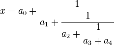
A classic example to see this in use is typesetting continued fractions (though it's better to use the \cfrac command^[1] described
in the Mathematics chapter over the method provided below). The following
code provides an example.

\begin{equation}   x = a_0 + \frac{1}{a_1 + \frac{1}{a_2 + \frac{1}{a_3 + a_4}}} \end{equation}

As you can see, as the fractions continue, they get smaller (although they will not get any smaller as in this example, they have reached the \scriptstyle limit).
If you wanted to keep the size consistent, you could declare each fraction to use the display style instead, e.g.:

\begin{equation}   x = a_0 + \frac{1}{\displaystyle a_1           + \frac{1}{\displaystyle a_2           + \frac{1}{\displaystyle a_3 + a_4}}} \end{equation}

Another approach is to use the \DeclareMathSizes command
to select your preferred sizes. You can only define sizes for \displaystyle, \textstyle,
etc. One potential downside is that this command sets the global maths sizes, as it can only be used in the document preamble.

However, it's fairly easy to use: \DeclareMathSizes{ds}{ts}{ss}{sss},
where ds is the display size, ts is the text size, etc. The values you input are assumed to be point (pt) size.

NB the changes only take place if the value in the first argument matches the current document text size. It is therefore common to see a set of declarations in the preamble, in the event of
the main font being changed. E.g.,

\DeclareMathSizes{10}{18}{12}{8}   % For size 10 text \DeclareMathSizes{11}{19}{13}{9}   % For size 11 text \DeclareMathSizes{12}{20}{14}{10}  % For size 12 text

[edit]Forcing
\displaystyle for all math in a document

Put

\everymath{\displaystyle}

before \begin{document} to force all math to \displaystyle.

To do: Consider to add stuff from mathtools

[edit]Notes

1. ↑ ^{a b c d e f g h i j k l m n o} Requires
   the amsmath package
2. ↑ ^a b c d requires
   the mathtools package