1.
[Measures].[Sales Sum] / [Measures].[Item Count]
If you need to take a simple average of values associated with a set of cells,
you can use the MDX Avg() function, as in the following example:
WITH
SET [My States] AS
‘{ [Customer].[MA], [Customer].[ME], [Customer].[MI], [Customer].[MO] }’
MEMBER [Customer].[Avg Over States] AS ‘Avg ([My States])’
SELECT
{ [Measures].[Dollar Sales], [Measures].[Unit Sales] } on columns,
{ [Products].[Family].Members } on rows
FROM Sales
WHERE ([Customer].[Avg Over States])
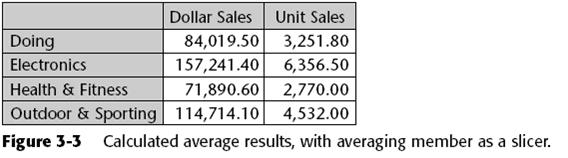
This query returns a grid of three measures by N product families. The sales, units, and profit measures are each averaged over the five best customers in terms of total profit. Notice that the expression to be averaged by the Avg() function has been left unspecified in the [Avg Over States] calculation. Leaving it unspecified is the equivalent of saying:
([Measures].CurrentMember, [Products].CurrentMember , . . . )
2.
Sum (
CrossJoin(
Descendants ([Industry].CurrentMember, [Industry].[Company],
SELF),
Descendants ([Time].CurrentMember, [Time].[Day], SELF)
)
,([Measures].[Share Price] * [Measures].[Units Sold])
) / [Measures].[Units Sold]
will calculate this weighted average.
A difficulty lurks in formulating the query this way, however. The greater the number of dimensions you are including in the average, the larger the size of the cross-joined set. You can run into performance problems (as well as intelligibility problems) if the number of dimensions being combined is large and the server actually builds the cross-joined set in memory while executing this. Moreover, you should account for all dimensions in the cube or you may accidentally involve aggregate [Share Price] values in a multiplication, which will probably be an error. In Analysis Services 2005, you can improve this by using NonEmpty() around a cross-join, as follows:
NonEmpty (
{ [Measures].[Share Price], [Measures].[Units Sold])}
* Descendants ([Industry].CurrentMember,
[Industry].[Company], SELF)
* Descendants ([Time].CurrentMember, [Time].[Day], SELF)
* Descendants ([Customer].CurrentMember, [Time].[Day], SELF))
)
3. 同比(时间)
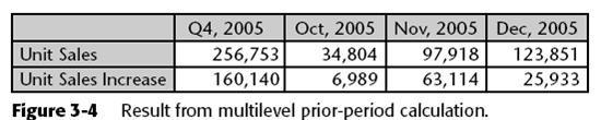
The following is equally valid, and its results are shown in Figure 3-4. Note that the Q4 difference is based on Q3 and Q4 expenses, whereas each month’s difference is based on its expenses and the prior month’s expenses.
WITH MEMBER [Measures].[Unit Sales Increase] AS
‘[Measures].[Unit Sales]
- ([Measures].[Unit Sales], [Time].CurrentMember.PrevMember)’
SELECT
{ [Time].[Q4, 2005], [Time].[Q4, 2005].Children } on columns,
{ [Measures].[Unit Sales], [Measures].[Unit Sales Increase] }
on rows
FROM Sales
4. 环比
PeriodsToDate ( [Time].[Year], [Time].CurrentMember ),
[Measures].[Dollar Sales]
)’
SELECT
{ [Time].[Quarter].[Q3, 2000], [Time].[Quarter].[Q4, 2000],
[Time].[Quarter].[Q1, 2001]
} on columns,
{ [Measures].[Expenses], [Measures].[YTD Expenses] } on rows
FROM Costing
Note that the [Unit Sales YAgo Increase] for Q1, 2005 is the difference
in first-quarter sales, whereas the [Unit Sales YAgo Increase] for Jan,
2005 is the difference in January sales.
5. Year-to-Date (Period-to-Date) Aggregations
WITH MEMBER [Measures].[YTD Dollar Sales] AS
‘Sum (
PeriodsToDate ( [Time].[Year], [Time].CurrentMember ),
[Measures].[Dollar Sales]
)’
SELECT