opencv 笔记08Core_DFT

现在的位置: 首页 > 综合 > 正文

opencv 笔记08Core_DFT

2013年10月06日 ⁄ 综合 ⁄ 共 5792字 ⁄ 字号小中大 ⁄ 评论关闭

#include "opencv2/core/core.hpp"
#include "opencv2/imgproc/imgproc.hpp"
#include "opencv2/highgui/highgui.hpp"
#include <iostream>
int main(int argc, char ** argv)
{
    const char* filename = argc >=2 ? argv[1] : "lena.jpg";

    Mat I = imread(filename, CV_LOAD_IMAGE_GRAYSCALE);
    if( I.empty())
        return -1;
    
    Mat padded;                            //expand input image to optimal size
    int m = getOptimalDFTSize( I.rows );
    int n = getOptimalDFTSize( I.cols ); // on the border add zero values
    copyMakeBorder(I, padded, 0, m - I.rows, 0, n - I.cols, BORDER_CONSTANT, Scalar::all(0));

    Mat planes[] = {Mat_<float>(padded), Mat::zeros(padded.size(), CV_32F)};
    Mat complexI;
    merge(planes, 2, complexI);         // Add to the expanded another plane with zeros

    dft(complexI, complexI);            // this way the result may fit in the source matrix

    // compute the magnitude and switch to logarithmic scale
    // => log(1 + sqrt(Re(DFT(I))^2 + Im(DFT(I))^2))
    split(complexI, planes);                   // planes[0] = Re(DFT(I), planes[1] = Im(DFT(I))
    magnitude(planes[0], planes[1], planes[0]);// planes[0] = magnitude  
    Mat magI = planes[0];
    
    magI += Scalar::all(1);                    // switch to logarithmic scale
    log(magI, magI);

    // crop the spectrum, if it has an odd number of rows or columns
    magI = magI(Rect(0, 0, magI.cols & -2, magI.rows & -2));

    // rearrange the quadrants of Fourier image  so that the origin is at the image center        
    int cx = magI.cols/2;
    int cy = magI.rows/2;

    Mat q0(magI, Rect(0, 0, cx, cy));   // Top-Left - Create a ROI per quadrant 
    Mat q1(magI, Rect(cx, 0, cx, cy));  // Top-Right
    Mat q2(magI, Rect(0, cy, cx, cy));  // Bottom-Left
    Mat q3(magI, Rect(cx, cy, cx, cy)); // Bottom-Right

    Mat tmp;                           // swap quadrants (Top-Left with Bottom-Right)
    q0.copyTo(tmp);
    q3.copyTo(q0);
    tmp.copyTo(q3);

    q1.copyTo(tmp);                    // swap quadrant (Top-Right with Bottom-Left)
    q2.copyTo(q1);
    tmp.copyTo(q2);

    normalize(magI, magI, 0, 1, CV_MINMAX); // Transform the matrix with float values into a 
                                            // viewable image form (float between values 0 and 1).

    imshow("Input Image"       , I   );    // Show the result
    imshow("spectrum magnitude", magI);    
    waitKey();

    return 0;
}

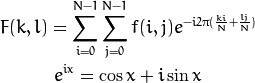
任一函数都可以表示成无数个正弦和余弦函数的和的形式。傅立叶变换就是一个用来将函数分解的工具。 2维图像的傅立叶变换可以用以下数学公式表达:

$F(k,l) = \displaystyle\sum\limits_{i=0}^{N-1}\sum\limits_{j=0}^{N-1} f(i,j)e^{-i2\pi(\frac{ki}{N}+\frac{lj}{N})}e^{ix} = \cos{x} + i\sin {x}$

式中 f 是空间域(spatial domain)值， F 则是频域(frequency domain)值。转换之后的频域值是复数，因此，显示傅立叶变换之后的结果需要使用实数图像(real image) 加虚数图像(complex image), 或者幅度图像(magitude
image)加相位图像(phase image)。在实际的图像处理过程中，仅仅使用了幅度图像，因为幅度图像包含了原图像的几乎所有我们需要的几何信息。

操作过程：

将图像延扩到最佳尺寸. 离散傅立叶变换的运行速度与图片的尺寸息息相关。当图像的尺寸是2， 3，5的整数倍时，计算速度最快。因此，为了达到快速计算的目的，经常通过添凑新的边缘像素的方法获取最佳图像尺寸。函数 getOptimalDFTSize() 返回最佳尺寸，而函数 copyMakeBorder() 填充边缘像素:

Mat padded;                            //将输入图像延扩到最佳的尺寸
int m = getOptimalDFTSize( I.rows );
int n = getOptimalDFTSize( I.cols ); // 在边缘添加0
copyMakeBorder(I, padded, 0, m - I.rows, 0, n - I.cols, BORDER_CONSTANT, Scalar::all(0));

添加的像素初始化为0.

C++: void copyMakeBorder(InputArray src,
OutputArray dst, int top, int bottom,
int left, int right, int borderType,
const Scalar& value=Scalar() )

Parameters:

Parameters:	src – Source image. dst – Destination image of the same type as `src` and the size `Size(src.cols+left+right,src.rows+top+bottom)` . top – bottom – left – right – Parameter specifying how many pixels in each direction from the source image rectangle to extrapolate. For example, `top=1, bottom=1, left=1, right=1` mean that 1 pixel-wide border needs to be built. borderType – Border type. See `borderInterpolate()` for details. value – Border value if `borderType==BORDER_CONSTANT` .

src – Source image.
dst – Destination image of the same type as src and
the size Size(src.cols+left+right,src.rows+top+bottom) .
top –
bottom –
left –
right – Parameter specifying how many pixels in each direction from the source image rectangle to extrapolate. For example, top=1, bottom=1, left=1, right=1 mean
that 1 pixel-wide border needs to be built.
borderType – Border type. See borderInterpolate() for
details.
value – Border value if borderType==BORDER_CONSTANT .

为傅立叶变换的结果(实部和虚部)分配存储空间. 傅立叶变换的结果是复数，这就是说对于每个原图像值，结果是两个图像值。此外，频域值范围远远超过空间值范围，因此至少要将频域储存在 float 格式中。结果我们将输入图像转换成浮点类型，并多加一个额外通道来储存复数部分：

Mat planes[] = {Mat_<float>(padded), Mat::zeros(padded.size(), CV_32F)};
Mat complexI;
merge(planes, 2, complexI);         // 为延扩后的图像增添一个初始化为0的通道

C++: void merge(const Mat* mv, size_t count, OutputArray dst)

C++: void merge(InputArrayOfArrays mv, OutputArray dst

Parameters:

mv –

 input array or vector of matrices to be merged; all the matrices in mv must

 have the same size and the same depth.
count – number of input matrices when mv is a plain

 C array; it must be greater than zero.
dst – output array of the same size and the same depth as mv[0];

 The number of channels will be the total number of channels in the matrix array.

Parameters:	mv – input array or vector of matrices to be merged; all the matrices in `mv` must have the same size and the same depth. count – number of input matrices when `mv` is a plain C array; it must be greater than zero. dst – output array of the same size and the same depth as `mv[0]`; The number of channels will be the total number of channels in the matrix array.

进行离散傅立叶变换. 支持图像原地计算 (输入输出为同一图像):

dft(complexI, complexI);            // 变换结果很好的保存在原始矩阵中

将复数转换为幅度.复数包含实数部分(Re)和复数部分 (imaginary - Im)。离散傅立叶变换的结果是复数，对应的幅度可以表示为:

$M = \sqrt[2]{ {Re(DFT(I))}^2 + {Im(DFT(I))}^2}$

转化为OpenCV代码:

split(complexI, planes);                   // planes[0] = Re(DFT(I), planes[1] = Im(DFT(I))
magnitude(planes[0], planes[1], planes[0]);// planes[0] = magnitude
Mat magI = planes[0];

C++: void magnitude(InputArray x, InputArray y, OutputArray magnitude)


Parameters:

x –

 floating-point array of x-coordinates of the vectors.
y – floating-point array of y-coordinates of the vectors; it must have the same size as x.
magnitude – output array of the same size and type as x.

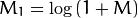
Parameters:	x – floating-point array of x-coordinates of the vectors. y – floating-point array of y-coordinates of the vectors; it must have the same size as `x`. magnitude – output array of the same size and type as `x`. $\texttt{dst} (I) = \sqrt{\texttt{x}(I)^2 + \texttt{y}(I)^2}$

对数尺度(logarithmic scale)缩放. 傅立叶变换的幅度值范围大到不适合在屏幕上显示。高值在屏幕上显示为白点，而低值为黑点，高低值的变化无法有效分辨。为了在屏幕上凸显出高低变化的连续性，我们可以用对数尺度来替换线性尺度:

$M_1 = \log{(1 + M)}$

转化为OpenCV代码:
```
magI += Scalar::all(1);                    // 转换到对数尺度
log(magI, magI);
```

剪切和重分布幅度图象限. 还记得我们在第一步时延扩了图像吗? 那现在是时候将新添加的像素剔除了。为了方便显示，我们也可以重新分布幅度图象限位置(注：将第五步得到的幅度图从中间划开得到四张1/4子图像，将每张子图像看成幅度图的一个象限，重新分布即将四个角点重叠到图片中心)。这样的话原点(0,0)就位移到图像中心。

magI = magI(Rect(0, 0, magI.cols & -2, magI.rows & -2));
int cx = magI.cols/2;
int cy = magI.rows/2;

Mat q0(magI, Rect(0, 0, cx, cy));   // Top-Left - 为每一个象限创建ROI
Mat q1(magI, Rect(cx, 0, cx, cy));  // Top-Right
Mat q2(magI, Rect(0, cy, cx, cy));  // Bottom-Left
Mat q3(magI, Rect(cx, cy, cx, cy)); // Bottom-Right

Mat tmp;                           // 交换象限 (Top-Left with Bottom-Right)
q0.copyTo(tmp);
q3.copyTo(q0);
tmp.copyTo(q3);

q1.copyTo(tmp);                    // 交换象限 (Top-Right with Bottom-Left)
q2.copyTo(q1);
tmp.copyTo(q2);

归一化. 这一步的目的仍然是为了显示。现在我们有了重分布后的幅度图，但是幅度值仍然超过可显示范围[0,1] 。我们使用 normalize() 函数将幅度归一化到可显示范围。

normalize(magI, magI, 0, 1, CV_MINMAX); // 将float类型的矩阵转换到可显示图像范围
                                        // (float [0， 1]).

C++: void normalize(InputArray src,
OutputArray dst, double alpha=1, double beta=0,
int norm_type=NORM_L2, int dtype=-1, InputArray mask=noArray() )

Parameters:

Parameters:	src – input array. dst – output array of the same size as `src` . alpha – norm value to normalize to or the lower range boundary in case of the range normalization. beta – upper range boundary in case of the range normalization; it is not used for the norm normalization. normType – normalization type (see the details below). dtype – when negative, the output array has the same type as `src`; otherwise, it has the same number of channels as `src` and the depth `=CV_MAT_DEPTH(dtype)`. mask – optional operation mask.

src – input array.
dst – output array of the same size as src .
alpha – norm value to normalize to or the lower range boundary in case of the range normalization.
beta – upper range boundary in case of the range normalization; it is not used for the norm normalization.
normType – normalization type (see the details below).
dtype – when negative, the output array has the same type as src;
otherwise, it has the same number of channels as src and the depth =CV_MAT_DEPTH(dtype).
mask – optional operation mask.