上篇文章提及的统计过程控制图是单一变量的控制图,它属于单值控制图。控制图的种类很多,我的老师在其书中如是分类:
(1)计量控制。对于产品的物理度量指标,如机器零件的尺寸,棉卷的重量,青砖的抗压强度等,在生产过程处于控制状态时,产品质量服从正态分布。根据这种指标进行抽样控制叫计量控制。常用的计量控制图有:单值控制图(即x控制图)、平均值控制图(即 控制图)、极差控制图(即R控制图)、中位数极差控制图(即 -R控制图)等。
(2)计件控制。产品中具有某种标志的产品件数指标,如一批产品中的次品件数、废品件数、一等品件数等,服从二项分布。根据这种指标进行抽样控制叫计数控制。常用的计数控制图有不合格品数控制图(即Pn控制图)和不合格品率控制图(即P控制图)等。
(3)计点控制。对于产品上的疵点数,比如一件铸件表面的孔、砂眼等,一匹布上的挑纱、竹节、破眼等,均服从普哇松分布。根据这种指标进行的抽样控制叫计点控制图。常用的计点控制图有缺陷数控制图(即C控制图)和单位缺陷控制图(即 控制图)。
这里涉及不同的分布函数,其中,正态分布中存在均值和方差,二项分布中的概率,普哇松分布(Poisson) 的参数λ。三种分布对应存在着X-R,X-S,P,PN,C,U等控制图,控制图的控制线对应着相应的等式. 以二项分布为例,其控制线公式为:

minitab软件画统计过程控制图很方便,该软件有以上几种控制图菜单操作,简单易行。大伙可以在MINITAB软件的工具栏找到统计(S),进而进入控制图(C),控制图下拉菜单里存在具体的控制图。例如,X-R控制图的界面:

sas软件在统计过程控制运用方面专门有个模块:QC模块,该模块除了可以进行统计过程控制的功能外,还可以用来进行质量改进、实验设计、工艺改进、分析统计过程能力、开发和评估抽样计划等。就统计过程控制图来说,QC模块支持一下语句来完成相应图形。
BOXCHART box chart with optional trend chart
CCHART c chart
IRCHART individual and moving range charts
MCHART median chart with optional trend chart
MRCHART median and R charts
NPCHART np chart
PCHART p chart
RCHART R chart
SCHART s chart
UCHART u chart
XCHART X chart with optional trend chart
XRCHART X and R charts
XSCHART X and s charts
另外,SAS/QC User's Guede有详细信息,部分控制图案例摘录如下:
/*Example 13.8: Applying Tests for Special Causes*/
data Trucks3;
input TruckID $ Defects @@;
label TruckID='Truck Identification Number'
Defects='Number of Paint Defects';
datalines;
B1 12 B2 4 B3 4 B4 3
B5 4 D1 2 D2 3 D3 3
D4 2 D9 4 M2 9 M6 13
L3 5 L4 4 L7 6 Z1 15
Z2 8 Z3 9 Z7 6 Z9 8
;
run;
ods graphics on;
title1 'c Chart for Paint Defects in New Trucks';
title2 'Tests=1 to 4';
proc shewhart data=Trucks3;
cchart Defects*TruckID / tests = 1 to 4
testlabel1 = 'Test=1 Signaled'
testlabel2 = 'Test=2 signaled'
odstitle = title
zonelabels
tabletests
tablelegend;
run;
ods graphics off;
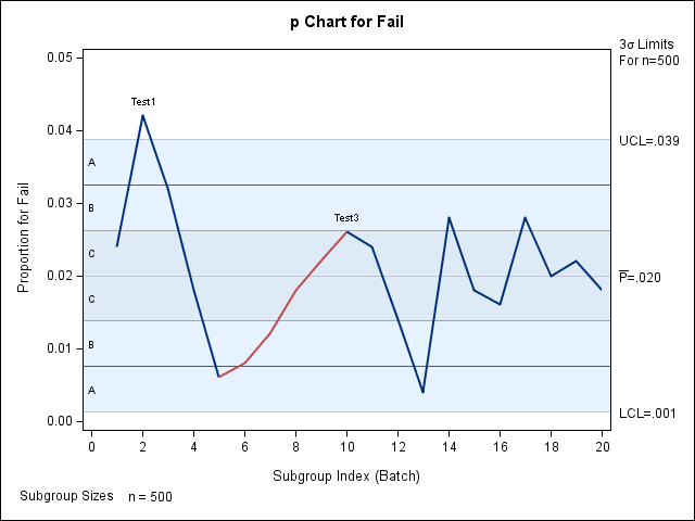
/*Example 13.22: Applying Tests for Special Causes*/
data Circuit3;
input Batch Fail @@;
datalines;
1 12 2 21 3 16 4 9
5 3 6 4 7 6 8 9
9 11 10 13 11 12 12 7
13 2 14 14 15 9 16 8
17 14 18 10 19 11 20 9
;
run;
ods graphics on;
title1'p Chart for the Proportion of Failing Circuits';
title2 'Tests = 1 to 4';
proc shewhart data=Circuit3;
pchart Fail*Batch / subgroupn = 500
tests = 1 to 4
zones
zonelabels
ltests = 20
table
tabletest
tablelegend;
run;
/*Example 13.31: Applying Tests for Special Causes*/
data Fabric3;
input Roll Defects @@;
datalines;
1 6 2 9 3 14 4 17
5 3 6 8 7 9 8 2
9 14 10 1 11 3 12 5
13 6 14 9 15 10 16 12
17 11 18 4 19 9 20 4
;
run;
ods graphics on;
title1 'u Chart for Fabric Defects';
title2 'Tests=1 to 4';
proc shewhart data=Fabric3;
uchart Defects*Roll / subgroupn = 30
tests = 1 to 4
odstitle = title
odstitle2 = title2
tabletests
zonelabels;
run;
ods graphics off;
/*Example 13.38: Applying Tests for Special Causes*/
data Tape;
input Sample $ WeightX WeightR;
WeightN=5;
label WeightX = 'Average Adhesive Amount'
Sample = 'Sample Code';
datalines;
C9 1270 35
C4 1258 25
A7 1248 24
A1 1260 39
A5 1273 29
D3 1260 21
D6 1259 37
D1 1240 37
R4 1260 28
H7 1255 19
H2 1268 36
H6 1253 36
P4 1273 29
P9 1275 22
J7 1257 24
J2 1269 41
J3 1249 36
B2 1264 31
G4 1258 25
G6 1248 36
G3 1248 30
;
run;
title 'Tests for Special Causes Applied to Adhesive Tape Data';
ods graphics on;
proc shewhart history=Tape;
xrchart Weight*Sample / tests = 1 to 5
odstitle = title
tabletests
zonelabels;
run;
ods graphics off;
title 'Tests for Special Causes Applied to Adhesive Tape Data';
proc shewhart history=Tape;
xrchart Weight*Sample / tests = 1 to 5
odstitle = title
tabletests
nochart
zonelabels;
run;
结果如下:


minitab也可以完成上述操作,但具体细节上有所差别,下面是minitab的控制图结果:


